Second degree equations with real coefficients

Since a long time ago, mathematicians have shown strong interest in solving second degree equations (also known as quadratic equations), i.e. equations for which the highest degree contains x2 (by using modern usual notations). Thus, the earliest known text referring to the latter dates back to two thousand years before our era, at the time of Babylonians. It is then Al-Khwarizmi, during the 9th century, who established the formulas for the systematic solving of these equations (please refer to the links given at the end of this post for the historical aspects).

Today, the methodology for solving second degree equations is based on their canonical form. For example, if we consider the equation x2 + 2x – 3 = 0, the trinomial x2 + 2x – 3 is like the beginning of a remarkable identity. Indeed, we can write:

x2 + 2x – 3
= x2 + 2x + 1 – 1 – 3
= x2 + 2x + 1 – 4
= (x+1)2 – 4, by recognizing a remarkable identity of the first type: (a+b)2 = a2 + 2ab + b2
= (x+1)2 – 22 which is the canonical form
= (x + 1 + 2)(x + 1 – 2), by recognizing this time a remarkable identity of the third type: a2 – b2 = (a+b)(a-b)
= (x + 3)(x – 1)

And at this point, we won :-) : by putting the factored trinomial back into our original equation, we obtain (x + 3)(x – 1) = 0.

We know that a product of terms is equal to zero if and only if at least one of the terms is equal to zero (this is due to the fact that zero is the absorbing element of the multiplication operation). This rule therefore leads to the system:


or

The two solutions are thus -3 et 1 (Yippee!)

We can crosscheck our result by plotting the graph of the function f(x) = x2 + 2x – 3. We can see that the resulting curve (a parabola) intersects the x-axis at two points that seem to have x = -3 and x = 1 as first coordinate (this is obviously not a proof but more a way to verify our methodology; on the other hand, our methodology is perfectly rigorous).

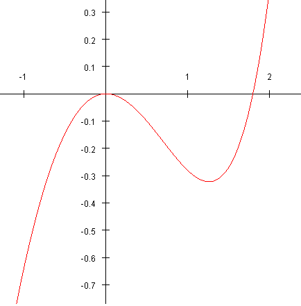
By still using curves to explore solutions, we can consider the following one. We can see here that the parabola never crosses the x-axis. So, the corresponding equation should have no solutions. Indeed, the equation is here x2 + 2x + 3 = 0. By repeating the previous methodology, we obtain:
x2 + 2x + 3
= x2 + 2x + 1 – 1 + 3
= (x+1)2 + 2

It is not possible to factor further this expression as we cannot find any remarkable identity! In fact, we have here two positive terms: (x+1)2, which is a power of 2 (thus positive) and 2 which is strictly positive. The sum of these two terms is always strictly positive and therefore never reaches zero. No solution!

We have to cover one last case, where the parabola is tangent to the x-axis (cutting it at just one point). This case corresponds to the equation x2-+2x+1 = 0 whose left-hand side is directly a remarkable identity, it thus transforms itself into (x+1)2 = 0 and the solution is x = -1 (sometimes referred to as a “double root”).

We are now ready to consider the generic problem of second degree equations solving. We will start with the trinomial ax2 + bx + c, assuming a is non-zero (to ensure that we really have a second degree here). We will proceed as before, and for this we start by factoring a:

To continue, we must assume that b2 – 4ac ⩾ 0. Under this assumption, a remarkable identity of the third type appears, leading to:


We must therefore consider the case a> 0 leading to √a2 = a and the case where a <0 giving √a2 = -a. In fact, we can see that both cases lead to the same result:

The equation is then and the solutions are:

These solutions are valid under the assumption we made, i.e. b2 – 4ac ⩾ 0 . For the particular case b2 – 4ac = 0, roots can be simplified as:

and it turns out that this is one and same root, corresponding to the case where the parabola cuts the x-axis at one point.

We are close to have finalized our analysis. We still have to consider the case where b2 – 4ac < 0. As it can be guessed, there is no solution: in , the term is strictly positive, forbidding any remarkable identity.

To summarize, by adopting the notation ∆ = b2 – 4ac (∆ is called the “discriminant” because its value allows to discriminate between the different possible results):

If ∆ > 0, the equation has two solutions, which are:

If ∆ = 0, a double root exists:

And if ∆ < 0, there are no real roots (we will not cover here imaginary solutions).

We have retrieved the three cases we highlighted in the first part of this post.

We have found Al-Khwarizmi’s solutions with a slightly faster method (because more general, see the Wikipedia article regarding this point). But we must also notice that we come some twelve centuries later!

References (for the historical aspects):
http://en.wikipedia.org/wiki/Quadratic_equation#History
http://www-history.mcs.st-and.ac.uk/HistTopics/Quadratic_etc_equations.html

Some thoughts about algorithms…

The notion of algorithm is not born with the first computers but well earlier, dating back to Antiquity. As commonly accepted, an algorithm is a set of instructions, a “recipe”, allowing reaching a predefined result. A systematic method can be seen as a synonym for algorithm, i.e. a way to surely reach a fixed goal (and with a finite number of operations). Considering this definition, a cooking recipe can be considered as being an algorithm (and some people are very talented for systematically spoiling their mayonnaise :-)) exactly like the music more played by a barrel organ reading perforated cards.

Euclide_enWell known examples of such systematic methods are the Sieve of Eratosthenes which determines the prime numbers smaller than a given N integer (N must obviously not be too big to allow the algorithm to converge in a reasonable time) or the Euclidean algorithm. The Euclidean algorithm (on the left side), which allows finding the Greatest Common Divisor of two integers, is noteworthy in the sense that it is much faster than the algorithm of successive subtractions, which is a method looking more “natural”, which first comes to mind.

The notion of algorithm is nowadays strongly linked with computers, these ogres of modern times which devour them without ever being sated. In this regard, it can be noted that French people use the word “informatique” for computer science, as the contraction of “automatic information”, which is a remarkable definition. Since operations performed by computer science are automatic, they rely necessarily on algorithms, which can be as simple as doing additions and subtractions in the case of cash registers (with very often a further refinement:  the generation of discount coupons valid for amounts slightly higher than your weekly purchases :-)) or can be very complex when it comes for example to the analysis of data extracted from billions of collisions occurring in particle accelerators.

The speed of an algorithm is an important factor in many cases. It is linked with the notion of real time. For example, the computer system that manages the entrance and exit of subway stations, depending in particular on the zone map, should give its verdict in just a second to ensure the smooth flow of travelers (waiting a minute would be totally unacceptable, causing massive human traffic jams every morning). In the same vein but on a different time scale, the computers forecasting the weather for the next day cannot afford a week of calculation (in this case, engineers adjust forecasting models based on the computing power of machines to be sure to get the results in a timely manner).

To be fast, an algorithm must be pertinent, i.e. it must be optimized. Let’s consider for example chess game. While in this game a human player relies on his experience and intuition (the latter often being unconscious experience), the machine will test a large number of moves by relying on its computing power to try to compete with the human player. The number of possible moves growing exponentially, calculations are optimized by pruning branches leading to situations with no interest. These enhancements, combined with the ever-increasing speed processing, allowed computers to compete with major international chess players and, at the beginning of this century, to beat them systematically.

This latest example shows that the methods deployed in the algorithms can be very different from those developed by human mind, even if, ultimately, the algorithms are (still!) designed by humans. If we push this thought a little bit further, should we not consider that life itself is just a big algorithm, a sequence of commands encoded in the DNA, with the objective of reproducing, at the molecular level, but also at the macroscopic scale, the living beings? Since millennia, bees follow a logic program optimized to ensure the survival of the community of the hive. And we, humans, are we programmed to seek happiness, find our soul mate and make babies with the unconscious objective to ensure the continuity of the human race? If yes, should we still consider ourselves as being free?

y = 3√[(16-x^2)/(2x+17)] and y = -3√[(16-x^2)/(2x+17)] what’s this ?

func
what is this?

 .

What a funny question! We can first do a study of the two associated functions.

 funcWe are told that the domain of definition of both functions is ]-∞ ;-17/2[ U [-4 ;4] and that the tables of variations are those on the left side (we can see here the differences, translated into “symmetries”, due to the minus sign).


But we still do not have a clear explanation! Let’s have a look at each curve.

func

They are both conforming to the previous tables of variations. It is possible to notice the horizontal tangents (and the symmetries already observed).


.

Let’s concentrate on the portion of curves from the interval [-4 ;4] and put them together on a unique graph.

func6

And then, if we add some colors …

func7

Happy Easter!

Source : http://www.mathematische-basteleien.de/eggcurves.htm

The intermediate value theorem reviewed

The intermediate value theorem is of great importance for functions analysis. It notably allows demonstrating that an equation has solutions even if they cannot be expressed. One form of this theorem says: “if a function f is defined and continuous on [a;b] then for every real number c belonging to [f(a);f(b)], the equation f(x) = c admits at least one solution”. The name of the theorem comes from the fact that it shows that all intermediate values c in [f(a);f(b)] are reached when sweeping [a;b].

The Bolzano theorem is proposing a simplified version of the previous theorem. It tells us that “if f(a) and f(b) are of opposite sign, which is equivalent to f(a)f(b) < 0, then the equation f(x) = 0 has at least one solution” (c, which is equal to 0 in this particular case, effectively belongs to [f(a);f(b)]).

The strength of the intermediate and Bolzano theorems is that their assumptions are applicable to all usual functions, which are all continuous at least on a sub-interval of their definition domain.

f : x↦ex-x2-x-1

These two theorems can easily be illustrated thanks to graphical representations. For example, let’s consider the function f : x↦ex-x2-x-1 drawn on the left side. It is easy to show that it is defined and continuous on [-1;2] and that f(-1)f(2) < 0. Consequently, the equation ex-x2-x-1 = 0 will have at least one solution in [-1;2]. In fact, as highlighted by the curve, there will be two solutions: 0 (evident solution) and a second one which cannot be expressed.

In order to prove the existence of a unique solution in a given interval, it is necessary to add a condition to the intermediate value theorem, known as corollary: “if furthermore the function is strictly monotonic on [a;b] (i.e. strictly increasing or strictly decreasing) then the equation f(x) = c, or f(x) = 0, admits a unique solution. We can for example apply this corollary to our function f: x↦ex-x2-x-1 on the interval [3/2;2].

table of variationsThe table of variations on the left side effectively shows us that the function f is strictly increasing on [3/2;2] and a calculator gives us easily f(3/2) < 0 and f(2) > 0. Consequently, the equation f(x) = 0 admits a unique solution on [3/2;2].

It is possible to reduce this interval by calculating for example f(7/4),   7/4 being the center of the interval [3/2;2]. The calculator says f(7/4) ≃ -0.058 < 0. Thus, the solution, very often designated as α, is as 7/4 < α < 2. By repeating this method, named  dichotomy, as  many times as needed, it is possible to get as near as wanted from α with the required accuracy. The dichotomy algorithm, which is painful to be run by hand, is usually programmed on a calculator or a computer, allowing getting an approximated value of α with several digits in less than a second. Other more sophisticated methods exist which are converging more quickly (i.e. they require less operations to reach the same accuracy) like Newton’s method of tangents. This method could be detailed in a coming post!